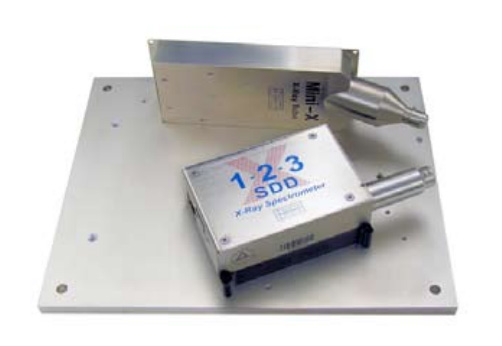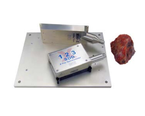
Amptek Quantitative Analysis Software for X-Ray Fluorescence XRF-FP

Amptek

XRF-FP is a quantitative analysis software package for X-Ray Fluoresence (XRF). XRF analysis with Fundamental Parameters (FP) converts elemental peak intensities to elemental concentrations or film thicknesses. It processes the raw X-ray spectra measured using Amptek’s detectors and signal processors to obtain (1) the elemental peak intensities (i.e., the intensity of the peaks corresponding to each element) and then (2) the elemental concentrations or film thicknesses.


立即咨詢
產(chǎn)品詳情


FEATURES
APPLICATIONS
? Fundamental parameters (FP)
? X-Ray Fluorescence
? Analysis with or without standards
? Thin-film Analysis
? General bulk and thin-film analysis
? RoHS/WEEE Analysis
? Analyze up to 40 elements
? Teaching and Research
? Supports all Amptek detectors (Si-PIN, Super
SDD, CdTe), X-ray tubes, and electronics
? Art and Archaeology
? Auto-mode for continuous or repeated analysis
? Process Control
? CdTe escape peak correction
? X-ray Tube Characterization
? Non-destructive analysis


XRF-FP is a quantitative analysis software package for X-Ray Fluoresence (XRF). XRF analysis with Fundamental Parameters (FP) converts elemental peak intensities to elemental concentrations or film thicknesses. It processes the raw X-ray spectra measured using Amptek’s detectors and signal processors to obtain (1) the elemental peak intensities (i.e., the intensity of the peaks corresponding to each element) and then (2) the elemental concentrations or film thicknesses.


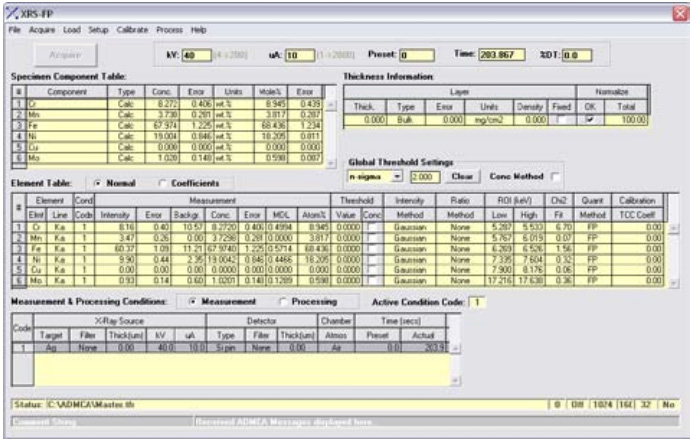
Figure 1: XRF-FP Main display window. Shows the element table with the various parameters and chemical concentrations.


XRF-FP SPECIFICATIONS
Introduction and Theory of Operation
   XRF-FP is a quantitative analysis software package for XRay Fluoresence (XRF). It processes the raw X-ray spectra measured using Amptek’s detectors and signal processors to obtain (1) the elemental peak intensities (i.e., the intensity of the peaks corresponding to each element) and then (2) the elemental concentrations or film thicknesses. There are three major steps to an XRF analysis, after the system has been setup and calibrated and the spectrum measured:
     1. Unravel the detector response to recover the incident photopeaks. This step corrects for the escape peaks, sum peaks, background continuum, background peaks, etc. The output of this step is a processed spectrum, ideally showing only the incident photopeaks.
     2. Deconvolve the photopeaks to determine the intensity of the X-rays interacting in the detector. The output of this step is a table of the intensities in each photopeak to be analyzed.
     3. Account for attenuation and matrix effects to determine the concentrations of the elements in the sample. The output of this step is a table of concentrations, which is the final result of the analysis.
   Spectrum processing corrects the spectrum for escape peaks, sum peaks, background continuum, Compton backscatter, and other effects. It also corrects for attenuation in the
Be window and detector dead layers and for the detector efficiency. It can fit the peaks using theoretical models or measured responses and can perform either a linear or a non-linear spectral deconvolution. The wide variety of processing options permits the software to be tailored to a particular detector/spectrometer and to particular
applications.
   Quantitative analysis, the step in which the element concentrations or film thicknesses are computed from the intensities, can be performed either standardless or using standards to calibrate the analytical parameters.
   With standardless analysis, all parameters are based upon theoretical equations, the fundamental parameter database, and precise modeling of the detector, X-ray tube, and
geometry. Standardless mode is possible for simple bulk or single-layer thin-film samples when the film thickness is known.
   With analysis using standards, the fundamental parameters are based on the measured response of the system for each element. The most accurate analytical results are obtained

NIST VALUE
XRS-FP VALUE
Steel316
CR
18.450 ± 0.05
18.500 ± 0.25
Mn
1.630 ± 0.01
1.670 ± 0.07
Fe
65.190 ± 0.07
65.000 ± 0.52
Ni
12.180 ± 0.05
12.270 ± 0.27
Cu
0.169 ± 0.001
0.167 ± 0.026
Mo
2.380 ± 0.01
2.390 ± 0.03
Steel321
Cr
17.400 ± 0.10
17.590 ± 0.23
Mn
1.800 ± 0.05
1.800 ± 0.07
Fe
69.310 ± 0.15
68.910 ± 0.53
Ni
11.200 ± 0.10
11.420 ± 0.27
Cu
0.121 ± 0.001
0.119 ± 0.022
Mo
0.165 ± 0.005
0.167 ± 0.009
Table 1. Results obtained using XRS-FP on two stainless steel alloys. These were “standard reference materials” from NIST. The data were taken using Amptek’s XR100-SDD detector with the PX4 signal processor, Amptek’s Mini-X X-ray tube, and Amptek’s MP1 mounting plate.


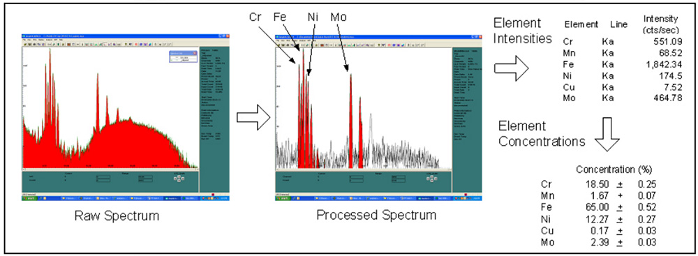
Figure 2. Sketch illustrating the data flow in an XRF analysis.


XRF-FP SPECIFICATIONS (con’t)
   using a “type” standard, a standard with composition similar to the material under measurement. Measured “scatter ratios” can be used to estimate the fraction of the sample which consists of low-Z materials that cannot be quantified by XRF.
   XRF-FP is a full-featured analytical software package which carries out these three steps. The software includes a large number of variables which the user can adjust to match the

experiment conditions and to optimize processing. 

XRF-FP Features

   ? Up to 40 elements can be analyzed at a time. Analysis can be performed for all elements from H through Fm, using K, L or M lines, in the energy range from 0.1 keV up to 60 keV.
   ? Supports measurement of bulk composition, composition and thickness of a single layer, or composition of up to 4 layers (for multi-layer call Amptek).
   ? Includes full correction for losses due to attenuation in air, detector Be windows, detector dead layers, the detector’s active volume, and filters inserted between the tube and sample or between the sample and detector. These are calculated from the user-input parameters
defining the excitation source, the detector, and the spectrometer geometry.
   ? Spectrum processing parameters include quantities to define the background continuum, pile-up and sum peaks, smoothing, a measured background spectrum for peaks
   ? Includes full corrections for absorption and both thick and thin-film secondary fluorescence, i.e., all matrix effects, enhancement and absorption. All possible lines are considered for both excitation and fluorescence.
   ? The photopeak intensity can be modeled as a Gaussian function, by integrating the net area of the peak, or using a measured reference photopeak response.
   ? Linear or nonlinear deconvolution. In nonlinear deconvolution, the centroid and resolution of the peaks is adjusted for the optimum fit.
   ? Quantitative analysis can be implemented using a pure fundamental parameters approach, fundamental parameters with scatter ratios (for samples containing large amounts of low-Z materials), or by simple least square fitting.
   ? Fundamental parameter analysis can be based on calibation from a single multielement standard, multiple standards, or no standards. Standardless analysis requires accurate definition of the tube, detector, environmental and geometry parameters.
   ? Fundamental parameter calculations are based upon the Sherman equation.
   ? Tube spectra can be supplied by the user or calculated from built-in models (Ebel, Pella et al.). These tube spectra can be convolved with experimental transfer functions to derive the expected tube spectrum passing through an optic such as a polycapillary bundle.

   ? Includes both an interactive “expert mode” and a “routine mode”. In expert mode, the user can see each step in the analysis and adjust parameters. In routine mode, after the spectrometer is set up and calibrated, one need only click a single button to acquire the data, process the spectrum, analyze the intensities, and save the output report.


Sample Definition
Elements/Components
   Can analyze up to 40 elements as individual elements and/or compounds. Unanalyzed elements can be specified stoichiometrically bound with an analyzed element (e.g., oxides or carbonates). Elements can be analyzed in one or more compounds within the same analysis. One compound (or element) can be analyzed by difference. Any number of compounds (or elements) can be “fixed.” For example, solutions, binders and/or hydrated crystals can be analyzed this way.
General Bulk and Thin-Film Analysis
   Any bulk or single-layer (unsupported) thin-film sample can be analyzed by either standardless or a calibration-with standards FP approach. Optional software is available to

handle multilayer samples up to 6 layers for simultaneous film thickness and composition analysis using FP with standards (please contact Amptek).


Quantitative Analysis
Analysis Method
   The analysis module includes three options: First, one can choose to use fundamental parameters (FP) for the quantitative analysis. This module solves a set of non-linear equations which relate the intensity of the X-ray peaks to the concentration of the elements in the sample. These equations include terms due to attenuation and enhancement in the sample, production of secondary X-rays in the sample, attenuation in windows and air, tube
spectra, scattering, etc.

   Second, one can choose FP with scatter ratios. This option is recommended when the sample contains a significant amount of low-Z materials, such as plastic. An estimate is made for the unanalyzed fraction of the sample by comparing the known fraction of analytes with the measured C/R ratio and ascribing the remainder to a pair of elements that bracket the estimated mean atomic number.

   Third, one can choose simple least squares fitting. This is empirical method, which does not use all the information about a sample. Instead, it relies on simple calibration coefficients and presumes that the intensity of a particular line is linearly related to the concentration.
   When more than one excitation is used, at least one of the elements for each condition must have been calibrated. Calibration factors may be generated using any type of standard (e.g., pure element or analytical “type” standard).A single “type” standard may be used, or the calibration may be done with a different standard for each element, or any combination of standards may be used. If some elements are calibrated and some are not, the latter can use
calibration coefficients derived from the former group.
   The mass thickness of the sample can either be specified or calculated. If the latter, then the analysis cannot be standardless. Several units are possible for thickness measurement, and the density can be calculated theoretically or specified in the case of linear thickness calculations.Composition units may be ppm or Wt%, with the additional output of atomic and mole percent.
Calibration Method
   With the FP analysis method, one can choose a “standardless” approach. All of the parameters describing the X-ray tube spectra, filtering, attenuation in air, attenuation in Be
windows and dead layers, attenuation and enhancement in the sample, etc. are computed from physical models based on the data the user has entered into the software. It is simple to use standardless analysis but the parameters are only approximate. This is due to approximations inherent in the physical models and in the data the user enters.
   With the FP analysis method, one can also choose to calibrate its parameters using either a single standard or multiple standards. Calibration is strongly recommended and will lead to much more accurate analysis results. A single “type” standard may be used, i.e. one can use a single piece of material containing all of the elements which will later be analyzed. For example, one can use a single “standard reference material” of stainless steel and then obtain very accurate analyses of other steel alloys. One can also calibrate with a different standard for each element.

   Several types of analysis cannot be standardless, i.e. calibration with standards (reference materials) is required.Least squares analysis cannot be standardless. If the mass thickness of the sample (i.e., the mg/cm2) is calculated, the analysis cannot be standardless. 

Excitation Sources

   Either X-ray tubes or isotopic sources can be used. For tubes, XRF-FP can model both reflection and transmission x-rays using either Pella or Ebel models, or via a supplied source spectrum for complete polychromatic source modeling. Tube anode, windows and filters may be specified. The tube window can be of any composition (e.g., BeO or glass). Any element may be chosen for the tube anode, as well as the tube (electron) incidence and take-off angles. The kV may range from 3 to 60 kV. Provision is provided for including a transmission efficiency file for use with, for example, polycapillary optics placed between the source
and the sample. Radioisotopes can be used using a sourcefile describing the relative line ratios. For secondary target excitation, monochromatic excitation is assumed.

   Amptek supplies all parameters for its Mini-X X-ray tube and filter kit. If a tube from a different vendor is used, then the customer must find the critical parameters. 

   Radioisotopes can be used using a source file describing the relative line ratios. For secondary target excitation,monochromatic excitation is assumed.

Detectors
   Various detectors (Si-PIN, SDD, CdTe, Si(Li), and Ge) and windows can be fully modeled. The software has provision for the user to input all the required parameters (e.g., thickness, are, dead layer, etc.) associated with these detectors and their windows. Spectral processing with CdTe involves some significant changes to the processing routines. For more information on CdTe detector analysis please see http://www.amptek.com/epeaks.html.
   Amptek supplies all the parameters for its XR100 series of detectors, including the XR100-SDD, XR100CR for SiPIN, and XR100-CdTe. If a detector from a different vendor is used, the customer must find the critical parameters.
Geometry
   The complete system geometry can be specified including the sample incidence and take-off angles, the source-to-optic and/or source-to-sample distances, the sample-to-detector distance, as well as the environmental factors. Amptek supplies all the parameters for its MP1 mounting plate, for use with the Mini-X and XR100/X-123.

Figure 3: Geometry angle definitions.


XRF-FP SPECIFICATIONS (con’t)


Figure 4. When using the MP1 mounting plate, refer to this diagram and the table below. The distance from the edge of the plate to the sample should be 0.375 inches (1 cm) in order to be at the intersecting point of the detector and x-ray tube. All dimensions are in centimeters
(cm).


XRF-FP Parameter
Value
Incidence Angle
67.5°
Take-Off Angle
67.5°
Alpha Angle
Scatter Angle
135°
Tube-to-sample
339 mm
Sample-to-detector
159 mm


Table 2.Whenusing the MP1 mountingplate with the XRF-FP software, enterthese values in the Geometry setup dialog.
Elements, Lines, and Interelement Corrections

   Includes full corrections for absorption and both thick and thin-film secondary fluorescence. All possible lines are considered for both excitation and fluorescence. The analysis can be performed for all elements from H through Fm, using K, L or M lines in the energy range from 0.1 keV up to 60 keV.


Spectrum Processing
Spectrum Calibration

   Using known peaks in the spectrum, the software calculates the effective gain (eV/channel) and offset (zero shift) for the spectrometer. These factors are applied to subsequent spectra prior to other spectrum processing. The calibration can be specified in the XRF-FP software or in the ADMCA software. XRF-FP can automatically import the calibration from ADMCA.

Background Removal and Blank Subtraction
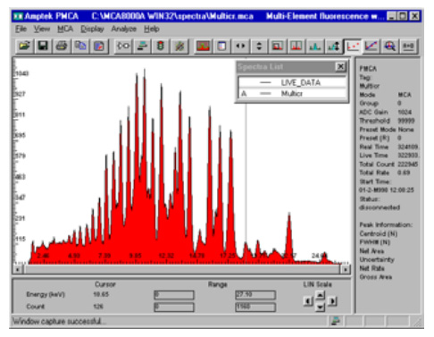
   The background removal module uses iterative filtering to distinguish peaks, leaving behind the smoothly varying spectral background. This background is then removed from the original spectrum, leaving the peaks.
   The blank subtraction module is used to remove peaks due to environmental interference or contamination. These peaks are not due to material in the sample but in the spectrometer, for example, Ar in the air or Al in the filters or Pb in a user’s shielding. This module subtracts a spectrum acquired from a “blank” reference material, i.e., one without the elements to be analyzed.


Figure 5: Original spectrum before background removal.
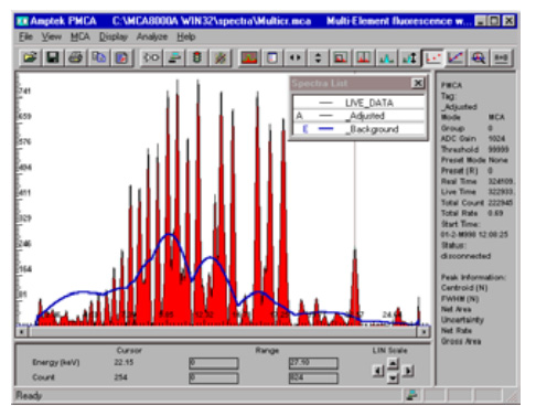
Figure 6. Processed spectrum and background. The blue curve
is the removed background.


Escape Peak and Sum Peak Removal

   Removes, at the user’s option, both detector escape and sum (pile-up) peaks. The escape peak module uses an internal function to estimate the fraction of x-ray events (above the K edge) that will generate K x-rays that will escape from the front or backside of the detector. Includes parameters for both Si and for CdTe.


XRF-FP SPECIFICATIONS (con’t)


   Please see http://www.amptek.com/epeaks.html for information on Escape Peak Corrections for CdTe detectors. This is important when characterizing the output X-ray spectrum of an X-ray tube or performing XRF with a CdTe detector.


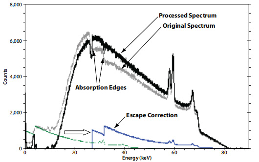
Figure 7. Plot showing a tungsten (W) X-ray tube output spectrum taken with a CdTe detector after processing to remove escape events. The gray trace shows the original spectrum. The
green trace illustrates the escape events in the original spectrum. These are subtracted from this original spectrum, then the correct energies are computed (by adding in the energy which escaped). The blue trace shows the corrected escape events, which are then summed with the gray trace. The dark black trace shows the final result of the processing with the events in their correct channels.


Smoothing
   A specified number of 1:2:1 Gaussian smooths can be applied to a spectrum.
Deconvolution: Intensity Extraction
   This module operates on the processed spectrum to extract the net peak intensities for the selected elements. It includes several options:
     First, the peak areas are computed using one of three methods: (1) simple peak integration across a fixed Region-Of-Interest, (2) fitting Gaussians to the peaks, using a known database of line ratios and peak energies, etc.,and (3) a reference deconvolution, which uses stored profiles for each element to fit the peaks.
     Second, the spectrum fitting can be done using either a linear or nonlinear approach. Both utilize a least-squares method. In linear fitting, the peak ratios, energies and widths are fixed. This method is usually very fast. In nonlinear fitting, these parameters are allowed to vary
within certain constraints. This method is much more computationally intensive.

   All required line energies and resolutions are calculated automatically from the specified analyte line. The Gaussian peak fitting can be done with a linear or non-linear leastsquares approach. The latter allows constrained changes in the peak positions, intra-series line ratios, and peak widths,from their nominal starting points.

   In addition to calculating elemental intensities, the software automatically calculates the estimated uncertainty and background values, which allows uncertainty and Minimum Detection Limit (MDL) calculations to be performed during the FP analysis.


Figure 8. Plot showing spectra from a stainless steel sample. The black trace is the raw spectrum, the blue trace is the processed spectrum, and the red curves show the result of a Gaussian deconvolution. The quantitative results are in Table 1.


Software Options
Spectrum Acquisition
   There are two methods of spectrum acquisition. The first is to acquire with the Amptek ADMCA acquisition application which controls the MCA8000A, DP5 Digital Pulse Processor, X-123, or PX5 Digital Processor and Power Supply. Once acquired, the XRF-FP can import the file and use the ADMCA display for spectrum processing. This is called “Expert Mode.”
   Once the system is set up and calibrated in “Expert Mode”, it can be used in “Routine Mode.” The user places the sample in the spectrometer, then in the screen in Figure 9 clicks “Analyze” and XRF-FP acquires the spectrum, saves it, analyzes it, and then saves the report. “Routine Mode” acquires the spectrum directly into the XRF-FP software which can then be automatically processed. A repeat measurement capability is provided.
Automatic Peak/Element ID
   Using the Amptek ADMCA application, the user can automatically mark peaks (ROIs) for analysis. If the appropriate element library is loaded into ADMCA the software will associate the marked peaks with elements. The corresponding elements can then be automatically
imported into XRF-FP element table.


Figure 9. Auto and Repeat Mode.


Advanced Description
   There are only two steps in XRF analysis whether or not the fundamental parameter (FP) method is used. The first step is to calibrate the response function for each element from one or many standards (called the “Calibration” step). The second step is to produce the sample analysis of a given material, using the previously stored calibration coefficients, and the FP algorithms given a definition of the sample (i.e., number of layers, and which elements are in
which layers).
   The software will support single layer or bulk composition and thickness analysis of up to 40 elements, calculated as either elements and/or compounds. Up to 4 or more excitation “conditions” are allowed per analysis. Each condition describes a separate analysis, and can be freely defined with any combination of experimental conditions, such as kV, tube anode, filter, detector filter, environment (air, vacuum, He) and acquisition time. This allows the analyst to measure some elements with one condition, and others completely differently, such that each analysis can be optimized for the specific element, or group of elements. Likewise, the spectrum processing steps can also be freely defined, and are all part of the condition code setup.
   The FP analysis software will support a single or multiple standard calibration scheme, or completely standardless analysis if the tube, detector, environmental and geometry parameters are known. Calibration standards should be passed one at a time and the merging of the calibration standard information is handled internally. After each calibration step, a set of calibration coefficients and associated information for each of the defined elements is returned,which can immediately be used if only one standard is employed. When using multiple calibration standards, all the coefficients are merged into one set, and then this final
set is available for subsequent quantitative analysis.
   The layer thicknesses must be fixed for standardless analysis. Results can be normalized to any value, and MUST be normalized for standardless analysis or when the layer thicknesses are calculated.
   Elements (or compounds) can be calculated, fixed, or determined by difference. Elements can also be determined by stoichiometry from the compound formulae. Composition results can be calculated in units of Wt% or ppm,and for thin films, units such as ug/cm2 and mg/cm2 are used for mass thickness. The latter can be converted to thickness (microns, microinches, nm, etc.) if the density is known. The density may be input or optionally calculated theoretically.
   All the appropriate FP calculations are made both during calibration and for Quantitation, using calculations based upon the Sherman equation. Tube spectra, required for the direct fluorescence calculations, can be supplied by the user or calculated from built-in models (Ebel, Pella et al.). These tube spectra can be convolved with experimental transfer functions to derive the expected tube spectrum passing through an optic such as a polycapillary bundle.
The presence of air paths will also be calculated from the input geometry parameters for both the source and detector paths. Single-element filters can also be inserted between the tube and the sample or between the sample and the detector, and the software can accommodate both.
   The detector parameters (window, thickness, area, etc.) will also be used to calculate the various absorption and efficiency effects when X-rays pass through the window and get deposited in the detector material. This is only strictly necessary when doing standardless analysis, but the calculations are always done this way for consistency, and to make it easier to compare calibration coefficients between elements. If the theory were perfect all the calibration coefficients would have the same value. In practice, differences should be relatively small, especially in comparison with coefficients that did not fully compensate for the detector
efficiencies. Usually when calibrating elements that all use the same line series (e.g., K), the coefficient variation is small (<30%), but is often larger when calibrating from mixed lines (e.g., K and L) because it is difficult to make absolute calculations that include the line series information (e.g., fluorescence yields).
   It is not necessary to collect pure-element spectra for FP analysis as no direct ratioing is necessary for the elemental intensities. The calculations are done this way to make it easier to do standardless analysis. Of course, it is possible to use pure-element standards if desired, and the complete FP calibration may be done this way without any “type” standards being used at all. This is useful if the analyst does not have type standards readily available. Both direct and secondary fluorescence effects are considered in the FP calculations. Included in the FP database are all the required parameters to calculate or recall absorption coefficients, fluorescence yields, jump factors, CosterKronig transitions, line energies, line ratios, transition
probabilities, etc.
   
The software consists of a main program window that provides the user interface. It runs on standard PCs (Windows XP and later) with at least 256MB RAM of memory. The XRF-FP software is completely compatible and integrated with the Amptek ADMCA display and acquisition software. It can also directly control all Amptek electronics to provide an auto/repeat/continuous mode of operations.


EXPERIMENTER’S XRF KITS


Experimenter’s XRF Kit with Si-PIN Includes:
Experimenter’s XRF Kit with SDD Includes:
? X-123 Complete Spectrometer with Si-PIN Detector (6 mm2/500 μm, 1 mil Be window)
? X-123 Complete Spectrometer with Super SDD (25 mm2/500 μm, 0.5 mil Be window)
? Mini-X USB Controlled X-Ray Tube
? XRF-FP Quantitative Analysis Software
? MP1 XRF Mounting Plate
? Stainless Steel 316 (SS316) test sample
? Complete documentation with step-by-step instructions
? Complete documentation with step-by-stepinstructions
? XRF Kit wizard for quick software setup


Figure 1: XRF-FP Main display window. Shows the element table with the various parameters and chemical concentrations.


XRF-FP SPECIFICATIONS
Introduction and Theory of Operation
   XRF-FP is a quantitative analysis software package for XRay Fluoresence (XRF). It processes the raw X-ray spectra measured using Amptek’s detectors and signal processors to obtain (1) the elemental peak intensities (i.e., the intensity of the peaks corresponding to each element) and then (2) the elemental concentrations or film thicknesses. There are three major steps to an XRF analysis, after the system has been setup and calibrated and the spectrum measured:
     1. Unravel the detector response to recover the incident photopeaks. This step corrects for the escape peaks, sum peaks, background continuum, background peaks, etc. The output of this step is a processed spectrum, ideally showing only the incident photopeaks.
     2. Deconvolve the photopeaks to determine the intensity of the X-rays interacting in the detector. The output of this step is a table of the intensities in each photopeak to be analyzed.
     3. Account for attenuation and matrix effects to determine the concentrations of the elements in the sample. The output of this step is a table of concentrations, which is the final result of the analysis.
   Spectrum processing corrects the spectrum for escape peaks, sum peaks, background continuum, Compton backscatter, and other effects. It also corrects for attenuation in the
Be window and detector dead layers and for the detector efficiency. It can fit the peaks using theoretical models or measured responses and can perform either a linear or a non-linear spectral deconvolution. The wide variety of processing options permits the software to be tailored to a particular detector/spectrometer and to particular
applications.
   Quantitative analysis, the step in which the element concentrations or film thicknesses are computed from the intensities, can be performed either standardless or using standards to calibrate the analytical parameters.
   With standardless analysis, all parameters are based upon theoretical equations, the fundamental parameter database, and precise modeling of the detector, X-ray tube, and
geometry. Standardless mode is possible for simple bulk or single-layer thin-film samples when the film thickness is known.
   With analysis using standards, the fundamental parameters are based on the measured response of the system for each element. The most accurate analytical results are obtained

NIST VALUE
XRS-FP VALUE
Steel316
CR
18.450 ± 0.05
18.500 ± 0.25
Mn
1.630 ± 0.01
1.670 ± 0.07
Fe
65.190 ± 0.07
65.000 ± 0.52
Ni
12.180 ± 0.05
12.270 ± 0.27
Cu
0.169 ± 0.001
0.167 ± 0.026
Mo
2.380 ± 0.01
2.390 ± 0.03
Steel321
Cr
17.400 ± 0.10
17.590 ± 0.23
Mn
1.800 ± 0.05
1.800 ± 0.07
Fe
69.310 ± 0.15
68.910 ± 0.53
Ni
11.200 ± 0.10
11.420 ± 0.27
Cu
0.121 ± 0.001
0.119 ± 0.022
Mo
0.165 ± 0.005
0.167 ± 0.009
Table 1. Results obtained using XRS-FP on two stainless steel alloys. These were “standard reference materials” from NIST. The data were taken using Amptek’s XR100-SDD detector with the PX4 signal processor, Amptek’s Mini-X X-ray tube, and Amptek’s MP1 mounting plate.


Figure 2. Sketch illustrating the data flow in an XRF analysis.


XRF-FP SPECIFICATIONS (con’t)
   using a “type” standard, a standard with composition similar to the material under measurement. Measured “scatter ratios” can be used to estimate the fraction of the sample which consists of low-Z materials that cannot be quantified by XRF.
   XRF-FP is a full-featured analytical software package which carries out these three steps. The software includes a large number of variables which the user can adjust to match the

experiment conditions and to optimize processing. 

XRF-FP Features

   ? Up to 40 elements can be analyzed at a time. Analysis can be performed for all elements from H through Fm, using K, L or M lines, in the energy range from 0.1 keV up to 60 keV.
   ? Supports measurement of bulk composition, composition and thickness of a single layer, or composition of up to 4 layers (for multi-layer call Amptek).
   ? Includes full correction for losses due to attenuation in air, detector Be windows, detector dead layers, the detector’s active volume, and filters inserted between the tube and sample or between the sample and detector. These are calculated from the user-input parameters
defining the excitation source, the detector, and the spectrometer geometry.
   ? Spectrum processing parameters include quantities to define the background continuum, pile-up and sum peaks, smoothing, a measured background spectrum for peaks
   ? Includes full corrections for absorption and both thick and thin-film secondary fluorescence, i.e., all matrix effects, enhancement and absorption. All possible lines are considered for both excitation and fluorescence.
   ? The photopeak intensity can be modeled as a Gaussian function, by integrating the net area of the peak, or using a measured reference photopeak response.
   ? Linear or nonlinear deconvolution. In nonlinear deconvolution, the centroid and resolution of the peaks is adjusted for the optimum fit.
   ? Quantitative analysis can be implemented using a pure fundamental parameters approach, fundamental parameters with scatter ratios (for samples containing large amounts of low-Z materials), or by simple least square fitting.
   ? Fundamental parameter analysis can be based on calibation from a single multielement standard, multiple standards, or no standards. Standardless analysis requires accurate definition of the tube, detector, environmental and geometry parameters.
   ? Fundamental parameter calculations are based upon the Sherman equation.
   ? Tube spectra can be supplied by the user or calculated from built-in models (Ebel, Pella et al.). These tube spectra can be convolved with experimental transfer functions to derive the expected tube spectrum passing through an optic such as a polycapillary bundle.

   ? Includes both an interactive “expert mode” and a “routine mode”. In expert mode, the user can see each step in the analysis and adjust parameters. In routine mode, after the spectrometer is set up and calibrated, one need only click a single button to acquire the data, process the spectrum, analyze the intensities, and save the output report.


Sample Definition
Elements/Components
   Can analyze up to 40 elements as individual elements and/or compounds. Unanalyzed elements can be specified stoichiometrically bound with an analyzed element (e.g., oxides or carbonates). Elements can be analyzed in one or more compounds within the same analysis. One compound (or element) can be analyzed by difference. Any number of compounds (or elements) can be “fixed.” For example, solutions, binders and/or hydrated crystals can be analyzed this way.
General Bulk and Thin-Film Analysis
   Any bulk or single-layer (unsupported) thin-film sample can be analyzed by either standardless or a calibration-with standards FP approach. Optional software is available to

handle multilayer samples up to 6 layers for simultaneous film thickness and composition analysis using FP with standards (please contact Amptek).


Quantitative Analysis
Analysis Method
   The analysis module includes three options: First, one can choose to use fundamental parameters (FP) for the quantitative analysis. This module solves a set of non-linear equations which relate the intensity of the X-ray peaks to the concentration of the elements in the sample. These equations include terms due to attenuation and enhancement in the sample, production of secondary X-rays in the sample, attenuation in windows and air, tube
spectra, scattering, etc.

   Second, one can choose FP with scatter ratios. This option is recommended when the sample contains a significant amount of low-Z materials, such as plastic. An estimate is made for the unanalyzed fraction of the sample by comparing the known fraction of analytes with the measured C/R ratio and ascribing the remainder to a pair of elements that bracket the estimated mean atomic number.

   Third, one can choose simple least squares fitting. This is empirical method, which does not use all the information about a sample. Instead, it relies on simple calibration coefficients and presumes that the intensity of a particular line is linearly related to the concentration.
   When more than one excitation is used, at least one of the elements for each condition must have been calibrated. Calibration factors may be generated using any type of standard (e.g., pure element or analytical “type” standard).A single “type” standard may be used, or the calibration may be done with a different standard for each element, or any combination of standards may be used. If some elements are calibrated and some are not, the latter can use
calibration coefficients derived from the former group.
   The mass thickness of the sample can either be specified or calculated. If the latter, then the analysis cannot be standardless. Several units are possible for thickness measurement, and the density can be calculated theoretically or specified in the case of linear thickness calculations.Composition units may be ppm or Wt%, with the additional output of atomic and mole percent.
Calibration Method
   With the FP analysis method, one can choose a “standardless” approach. All of the parameters describing the X-ray tube spectra, filtering, attenuation in air, attenuation in Be
windows and dead layers, attenuation and enhancement in the sample, etc. are computed from physical models based on the data the user has entered into the software. It is simple to use standardless analysis but the parameters are only approximate. This is due to approximations inherent in the physical models and in the data the user enters.
   With the FP analysis method, one can also choose to calibrate its parameters using either a single standard or multiple standards. Calibration is strongly recommended and will lead to much more accurate analysis results. A single “type” standard may be used, i.e. one can use a single piece of material containing all of the elements which will later be analyzed. For example, one can use a single “standard reference material” of stainless steel and then obtain very accurate analyses of other steel alloys. One can also calibrate with a different standard for each element.

   Several types of analysis cannot be standardless, i.e. calibration with standards (reference materials) is required.Least squares analysis cannot be standardless. If the mass thickness of the sample (i.e., the mg/cm2) is calculated, the analysis cannot be standardless. 

Excitation Sources

   Either X-ray tubes or isotopic sources can be used. For tubes, XRF-FP can model both reflection and transmission x-rays using either Pella or Ebel models, or via a supplied source spectrum for complete polychromatic source modeling. Tube anode, windows and filters may be specified. The tube window can be of any composition (e.g., BeO or glass). Any element may be chosen for the tube anode, as well as the tube (electron) incidence and take-off angles. The kV may range from 3 to 60 kV. Provision is provided for including a transmission efficiency file for use with, for example, polycapillary optics placed between the source
and the sample. Radioisotopes can be used using a sourcefile describing the relative line ratios. For secondary target excitation, monochromatic excitation is assumed.

   Amptek supplies all parameters for its Mini-X X-ray tube and filter kit. If a tube from a different vendor is used, then the customer must find the critical parameters. 

   Radioisotopes can be used using a source file describing the relative line ratios. For secondary target excitation,monochromatic excitation is assumed.
Detectors
   Various detectors (Si-PIN, SDD, CdTe, Si(Li), and Ge) and windows can be fully modeled. The software has provision for the user to input all the required parameters (e.g., thickness, are, dead layer, etc.) associated with these detectors and their windows. Spectral processing with CdTe involves some significant changes to the processing routines. For more information on CdTe detector analysis please see http://www.amptek.com/epeaks.html.
   Amptek supplies all the parameters for its XR100 series of detectors, including the XR100-SDD, XR100CR for SiPIN, and XR100-CdTe. If a detector from a different vendor is used, the customer must find the critical parameters.
Geometry
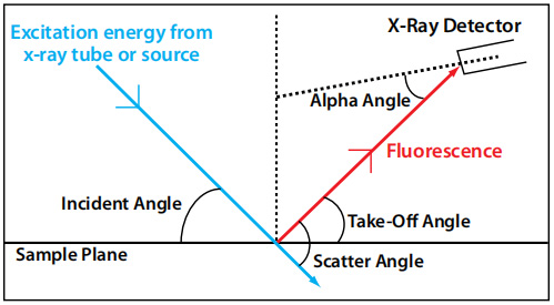
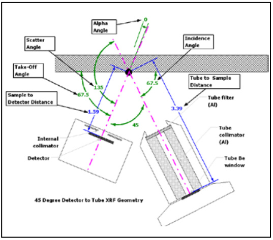
   The complete system geometry can be specified including the sample incidence and take-off angles, the source-to-optic and/or source-to-sample distances, the sample-to-detector distance, as well as the environmental factors. Amptek supplies all the parameters for its MP1 mounting plate, for use with the Mini-X and XR100/X-123.

Figure 3: Geometry angle definitions.

XRF-FP SPECIFICATIONS (con’t)

Figure 4. When using the MP1 mounting plate, refer to this diagram and the table below. The distance from the edge of the plate to the sample should be 0.375 inches (1 cm) in order to be at the intersecting point of the detector and x-ray tube. All dimensions are in centimeters
(cm).

XRF-FP Parameter
Value
Incidence Angle
67.5°
Take-Off Angle
67.5°
Alpha Angle
Scatter Angle
135°
Tube-to-sample
339 mm
Sample-to-detector
159 mm

Table 2.Whenusing the MP1 mountingplate with the XRF-FP software, enterthese values in the Geometry setup dialog.
Elements, Lines, and Interelement Corrections

   Includes full corrections for absorption and both thick and thin-film secondary fluorescence. All possible lines are considered for both excitation and fluorescence. The analysis can be performed for all elements from H through Fm, using K, L or M lines in the energy range from 0.1 keV up to 60 keV.


Spectrum Processing
Spectrum Calibration

   Using known peaks in the spectrum, the software calculates the effective gain (eV/channel) and offset (zero shift) for the spectrometer. These factors are applied to subsequent spectra prior to other spectrum processing. The calibration can be specified in the XRF-FP software or in the ADMCA software. XRF-FP can automatically import the calibration from ADMCA.


Background Removal and Blank Subtraction
   The background removal module uses iterative filtering to distinguish peaks, leaving behind the smoothly varying spectral background. This background is then removed from the original spectrum, leaving the peaks.
   The blank subtraction module is used to remove peaks due to environmental interference or contamination. These peaks are not due to material in the sample but in the spectrometer, for example, Ar in the air or Al in the filters or Pb in a user’s shielding. This module subtracts a spectrum acquired from a “blank” reference material, i.e., one without the elements to be analyzed.


Figure 5: Original spectrum before background removal.
Figure 6. Processed spectrum and background. The blue curve
is the removed background.


Escape Peak and Sum Peak Removal

   Removes, at the user’s option, both detector escape and sum (pile-up) peaks. The escape peak module uses an internal function to estimate the fraction of x-ray events (above the K edge) that will generate K x-rays that will escape from the front or backside of the detector. Includes parameters for both Si and for CdTe.


XRF-FP SPECIFICATIONS (con’t)


   Please see http://www.amptek.com/epeaks.html for information on Escape Peak Corrections for CdTe detectors. This is important when characterizing the output X-ray spectrum of an X-ray tube or performing XRF with a CdTe detector.


Figure 7. Plot showing a tungsten (W) X-ray tube output spectrum taken with a CdTe detector after processing to remove escape events. The gray trace shows the original spectrum. The
green trace illustrates the escape events in the original spectrum. These are subtracted from this original spectrum, then the correct energies are computed (by adding in the energy which escaped). The blue trace shows the corrected escape events, which are then summed with the gray trace. The dark black trace shows the final result of the processing with the events in their correct channels.


Smoothing
   A specified number of 1:2:1 Gaussian smooths can be applied to a spectrum.
Deconvolution: Intensity Extraction
   This module operates on the processed spectrum to extract the net peak intensities for the selected elements. It includes several options:
     First, the peak areas are computed using one of three methods: (1) simple peak integration across a fixed Region-Of-Interest, (2) fitting Gaussians to the peaks, using a known database of line ratios and peak energies, etc.,and (3) a reference deconvolution, which uses stored profiles for each element to fit the peaks.
     Second, the spectrum fitting can be done using either a linear or nonlinear approach. Both utilize a least-squares method. In linear fitting, the peak ratios, energies and widths are fixed. This method is usually very fast. In nonlinear fitting, these parameters are allowed to vary
within certain constraints. This method is much more computationally intensive.

   All required line energies and resolutions are calculated automatically from the specified analyte line. The Gaussian peak fitting can be done with a linear or non-linear leastsquares approach. The latter allows constrained changes in the peak positions, intra-series line ratios, and peak widths,from their nominal starting points.

   In addition to calculating elemental intensities, the software automatically calculates the estimated uncertainty and background values, which allows uncertainty and Minimum Detection Limit (MDL) calculations to be performed during the FP analysis.
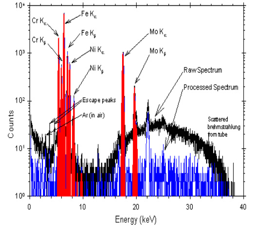
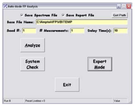
Figure 8. Plot showing spectra from a stainless steel sample. The black trace is the raw spectrum, the blue trace is the processed spectrum, and the red curves show the result of a Gaussian deconvolution. The quantitative results are in Table 1.


Software Options
Spectrum Acquisition
   There are two methods of spectrum acquisition. The first is to acquire with the Amptek ADMCA acquisition application which controls the MCA8000A, DP5 Digital Pulse Processor, X-123, or PX5 Digital Processor and Power Supply. Once acquired, the XRF-FP can import the file and use the ADMCA display for spectrum processing. This is called “Expert Mode.”
   Once the system is set up and calibrated in “Expert Mode”, it can be used in “Routine Mode.” The user places the sample in the spectrometer, then in the screen in Figure 9 clicks “Analyze” and XRF-FP acquires the spectrum, saves it, analyzes it, and then saves the report. “Routine Mode” acquires the spectrum directly into the XRF-FP software which can then be automatically processed. A repeat measurement capability is provided.
Automatic Peak/Element ID
   Using the Amptek ADMCA application, the user can automatically mark peaks (ROIs) for analysis. If the appropriate element library is loaded into ADMCA the software will associate the marked peaks with elements. The corresponding elements can then be automatically
imported into XRF-FP element table.


Figure 9. Auto and Repeat Mode.


Advanced Description
   There are only two steps in XRF analysis whether or not the fundamental parameter (FP) method is used. The first step is to calibrate the response function for each element from one or many standards (called the “Calibration” step). The second step is to produce the sample analysis of a given material, using the previously stored calibration coefficients, and the FP algorithms given a definition of the sample (i.e., number of layers, and which elements are in
which layers).
   The software will support single layer or bulk composition and thickness analysis of up to 40 elements, calculated as either elements and/or compounds. Up to 4 or more excitation “conditions” are allowed per analysis. Each condition describes a separate analysis, and can be freely defined with any combination of experimental conditions, such as kV, tube anode, filter, detector filter, environment (air, vacuum, He) and acquisition time. This allows the analyst to measure some elements with one condition, and others completely differently, such that each analysis can be optimized for the specific element, or group of elements. Likewise, the spectrum processing steps can also be freely defined, and are all part of the condition code setup.
   The FP analysis software will support a single or multiple standard calibration scheme, or completely standardless analysis if the tube, detector, environmental and geometry parameters are known. Calibration standards should be passed one at a time and the merging of the calibration standard information is handled internally. After each calibration step, a set of calibration coefficients and associated information for each of the defined elements is returned,which can immediately be used if only one standard is employed. When using multiple calibration standards, all the coefficients are merged into one set, and then this final
set is available for subsequent quantitative analysis.
   The layer thicknesses must be fixed for standardless analysis. Results can be normalized to any value, and MUST be normalized for standardless analysis or when the layer thicknesses are calculated.
   Elements (or compounds) can be calculated, fixed, or determined by difference. Elements can also be determined by stoichiometry from the compound formulae. Composition results can be calculated in units of Wt% or ppm,and for thin films, units such as ug/cm2 and mg/cm2 are used for mass thickness. The latter can be converted to thickness (microns, microinches, nm, etc.) if the density is known. The density may be input or optionally calculated theoretically.
   All the appropriate FP calculations are made both during calibration and for Quantitation, using calculations based upon the Sherman equation. Tube spectra, required for the direct fluorescence calculations, can be supplied by the user or calculated from built-in models (Ebel, Pella et al.). These tube spectra can be convolved with experimental transfer functions to derive the expected tube spectrum passing through an optic such as a polycapillary bundle.
The presence of air paths will also be calculated from the input geometry parameters for both the source and detector paths. Single-element filters can also be inserted between the tube and the sample or between the sample and the detector, and the software can accommodate both.
   The detector parameters (window, thickness, area, etc.) will also be used to calculate the various absorption and efficiency effects when X-rays pass through the window and get deposited in the detector material. This is only strictly necessary when doing standardless analysis, but the calculations are always done this way for consistency, and to make it easier to compare calibration coefficients between elements. If the theory were perfect all the calibration coefficients would have the same value. In practice, differences should be relatively small, especially in comparison with coefficients that did not fully compensate for the detector
efficiencies. Usually when calibrating elements that all use the same line series (e.g., K), the coefficient variation is small (<30%), but is often larger when calibrating from mixed lines (e.g., K and L) because it is difficult to make absolute calculations that include the line series information (e.g., fluorescence yields).
   It is not necessary to collect pure-element spectra for FP analysis as no direct ratioing is necessary for the elemental intensities. The calculations are done this way to make it easier to do standardless analysis. Of course, it is possible to use pure-element standards if desired, and the complete FP calibration may be done this way without any “type” standards being used at all. This is useful if the analyst does not have type standards readily available. Both direct and secondary fluorescence effects are considered in the FP calculations. Included in the FP database are all the required parameters to calculate or recall absorption coefficients, fluorescence yields, jump factors, CosterKronig transitions, line energies, line ratios, transition
probabilities, etc.
   
The software consists of a main program window that provides the user interface. It runs on standard PCs (Windows XP and later) with at least 256MB RAM of memory. The XRF-FP software is completely compatible and integrated with the Amptek ADMCA display and acquisition software. It can also directly control all Amptek electronics to provide an auto/repeat/continuous mode of operations.


EXPERIMENTER’S XRF KITS


Experimenter’s XRF Kit with Si-PIN Includes:
Experimenter’s XRF Kit with SDD Includes:
? X-123 Complete Spectrometer with Si-PIN Detector (6 mm2/500 μm, 1 mil Be window)
? X-123 Complete Spectrometer with Super SDD (25 mm2/500 μm, 0.5 mil Be window)
? Mini-X USB Controlled X-Ray Tube
? XRF-FP Quantitative Analysis Software
? MP1 XRF Mounting Plate
? Stainless Steel 316 (SS316) test sample
? Complete documentation with step-by-step instructions
? Complete documentation with step-by-stepinstructions
? XRF Kit wizard for quick software setup


Copyright? 安徽省科華貿(mào)易有限責(zé)任公司 版權(quán)所有 皖I(lǐng)CP備18022818號(hào)-1
地址:安徽省合肥市高新區(qū)昌河科創(chuàng)大廈702室電話:0551-65392835郵箱:service@kehua-trade.com
Designed by Wanhu
微信二維碼
国产成人亚洲影院,成人永久免费福利视频APP,成人女性爽爽影院,国外人成人色视频在线